Terrain Models and Triangulation
Once the point cloud has been prepared, it can be used directly in analyses or form the basis for a surface model. In many workflows, a triangulated model is established where the points are connected into a coherent triangle network.
Triangulation
Traditional terrain models are often based on the 2.5D principle, where each plan position can only have one height value. This works well for ordinary terrain surfaces, but is not sufficient for geometry with:
- overhangs
- vertical surfaces
- niches
- cuts and rock walls
- parts of tunnels and structures
Surface modeling extends this with 3D triangulation, where triangulation occurs in space and can represent more complex surfaces. This is important when the model needs to represent actual surfaces with greater geometric complexity than a conventional terrain model can handle.

3D triangulation of scanned point cloud
Gemini SurfaceMaker supports two different 3D triangulation methods for data in GMI layers:
The first method is a pure 3D triangulation and can be used for everything from scanned terrain models to structures.
Note
Gemini Terrain+ supports 2.5D triangulation.
3D Triangulation
To reconstruct surfaces from point clouds, a pure 3D triangulation method can be used. The function is found under Tools in the context menu in the map window.
It is important to pre-process the point clouds before 3D triangulation. Noise and other unwanted objects should be removed beforehand. Gemini Terrain has both manual methods for editing point clouds and an automatic method for removing noise.
The triangulation itself is normally performed in two or more iterations, but it is fully possible to run only the 1st iteration if a quick and rough triangulation is all that is needed.
Triangulation – 1st Iteration
In the first iteration, a cell size is specified to reduce the number of points in the triangulation. Based on the cell size, the algorithm selects an arbitrary point to represent each cell. What cell size is appropriate? This depends on the content of the scan. A rule of thumb is half the distance between two surfaces you want to distinguish. For example, if you scan both sides of a wall that is 50 cm thick, the cell size should be 0.25 or smaller. If you have many different types of areas, it may be sensible to split the point cloud to achieve the smallest possible triangle network.
In the first iteration, there are two additional options that can be useful. These are especially relevant for scan data with sharp edges, such as structures.
The first option is a statistical method where the program identifies probable edge points. Not all types of scans are suited for this method. A rock cut is a typical example of scan data where the geometry often makes this method unsuitable.
Another option is to include breaklines in the 3D triangulation. If the selection also contains 3D lines, this option becomes active in the dialog. The program simulates breaklines by generating dense points along the lines (point spacing equal to the accuracy). Breaklines can be surveyed with traditional land surveying or digitized directly in the point cloud. Note that this method must be used with caution – it is easy to introduce "noise" with this option.
Points from these additional options are included in the point selection before the 1st iteration triangulation is run.
Triangulation – 2nd Iteration
In the second step, the desired accuracy of the triangle network is set by specifying a value for Maximum distance from original points. All points in the original point cloud with a greater distance from the triangle network from the 1st iteration will be included in the point selection for triangulation.
This process can be repeated multiple times. The number of iterations is not specified directly; instead, a stop criterion is entered. The criterion is a percentage value for the number of points added compared to the original point set. The maximum number of iterations is set to 10.
Running multiple iterations is relevant when working with point clouds containing little noise. This can result in a model where no points fall outside the accuracy requirement. If the model contains noise, many iterations will cause more and more noise points to be included in the triangulation.
It is also possible to check the option to fill holes. This process runs after the last iteration. The criteria are Maximum perimeter and Maximum 3D area. The program first checks the hole's perimeter against the specified criterion. If the perimeter is smaller, the next criterion is checked. If the 3D area is also smaller than the criterion, the hole is filled. Both criteria must be met for a hole to be filled. Two criteria are used because square and rectangular holes can have approximately the same area but large differences in perimeter.
Result from Triangulation
The user determines where the result is placed using the Result application layer option. By default, the program suggests the active layer. Only application layers open for editing are listed in the dropdown menu.
Properties are assigned to the triangle network during triangulation:
| Attribute | Code | Description |
|---|---|---|
| S_JOBRESULT | S01 3D triangulated | Code value indicating how the triangle network was created |
| 3DTri_Cellstart | Cell size for simplification of triangle network | |
| 3DTri_MaxDist | Max. distance from original points (required accuracy) |
Example showing the effect of some settings on the result
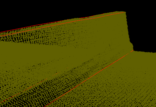
Cell size: 0.1
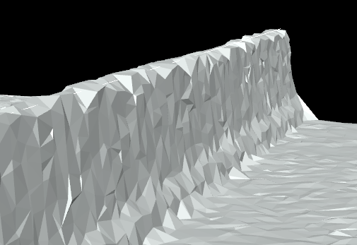
Required accuracy: 0.025
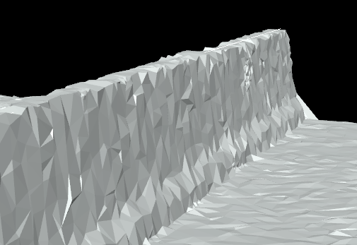
With probable edge points
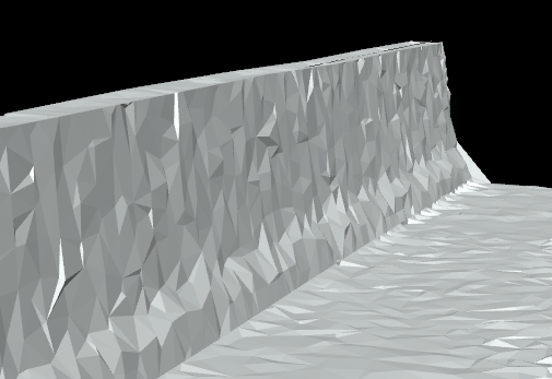
With breaklines
Triangulation of 3D Polygons
This triangulation tool also supports vertical polygons, as well as polygons with or without holes. Multiple polygons can be triangulated in one operation, and the function will merge the triangle networks into one object. If an existing triangle network is also included in the selection, a copy of it will be merged with the new ones.
The function is found under Tools in the horizontal list window for polygons.
Example of triangulation of 3D polygons
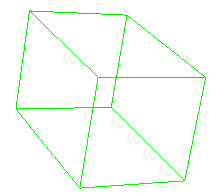
A starting point with six polygons:
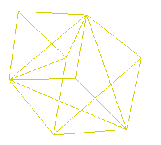
Produces a triangle network with volume:
Use of Terrain Models
Completed triangle networks and terrain models can be used for:
- volume calculation
- area calculation
- profile generation
- geometric control
- visualization
- design basis
- documentation of execution
It is generally important that the model type and triangulation method are chosen based on what the model will be used for. A model for visualization may have different requirements than one used for quantity calculations or machine control.